Viz - MPAS Tutorial

Intro¶

With unstructured-grid data, the grid/coordinate information is usually stored in a separate file from the model output fields. Considerably more information is needed to reconstruct the grid than in the case of a rectangular lat/lon grid, for example, which can be expressed with 1-D coordinate variables (e.g. ERA5).

With MPAS-A, the necessary grid variables are available in multiple files:

the grid file (usually ends in .grid.nc)
- agnostic to simulation
- note that with the standard limited-area workflow, which involves cutting out a section of a global grid, this can’t be used
the static file (usually ends in .static.nc)
- produced as part of the model initialization/prep process, contains static fields like terrain height
initial conditions (usually ends in .init.nc)
- easier to work with since the connectivity for the primal mesh uses zeros for padding

Some example grid and static files are available at: https://mpas-dev.github.io/atmosphere/atmosphere_meshes.html

Or on Casper/Derecho at:

/glade/campaign/mmm/wmr/duda/mesh/

Data¶

import os
from pathlib import Path

import cartopy.crs as ccrs
import cartopy.feature as cfeature
import geoviews.feature as gf
import geovista as gv
import matplotlib.pyplot as plt
import numpy as np
import pyvista as pv
import requests
import uxarray as ux
import xarray as xr

CI = os.environ.get("CI", "false").strip() == "true"

# https://docs.pyvista.org/user-guide/jupyter/
pv.set_jupyter_backend("static")

_ = xr.set_options(display_expand_data=False)

First we fetch an example global mesh: x1.2562 (~ 480-km resolution; chosen for its small file size and quickness to plot). Note that the uniform global meshes are really quasi-uniform.

def fetch_example_mesh(mesh: str = "x1.2562"):
    """Fetch example mesh from
    https://www2.mmm.ucar.edu/projects/mpas/atmosphere_meshes
    returning paths to the grid file and the static file."""
    import tarfile
    from io import BytesIO

    base = "https://www2.mmm.ucar.edu/projects/mpas/atmosphere_meshes"

    p_grid = Path(f"{mesh}.grid.nc")
    if not p_grid.is_file():
        r = requests.get(f"{base}/{mesh}.tar.gz", stream=True)
        r.raise_for_status()
        with tarfile.open(fileobj=BytesIO(r.content), mode="r:gz") as tar:
            tar.extract(p_grid.name, filter="data")

    p_static = Path(f"{mesh}.static.nc")
    if not p_static.is_file():
        r = requests.get(f"{base}/{mesh}_static.tar.gz", stream=True)
        r.raise_for_status()
        with tarfile.open(fileobj=BytesIO(r.content), mode="r:gz") as tar:
            tar.extract(p_static.name, filter="data")

    return p_grid, p_static

grid_path, _ = fetch_example_mesh()

g = xr.open_dataset(grid_path)
assert g.sphere_radius == 1, "unit sphere"

area = g.areaCell * 6371**2  # m2 on unit sphere -> km2 on Earth sphere
area.attrs.update(units="km2")

_, _, patches = np.sqrt(area).plot.hist(bins=20, size=3.5, aspect=1.8)
plt.xlabel("sqrt(areaCell) [km$^2$]")
plt.ylabel("Count")
_ = plt.bar_label(patches, size=8)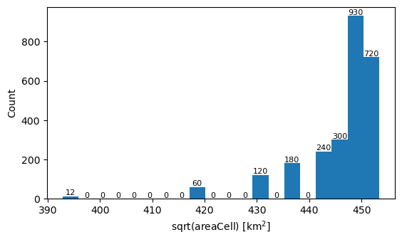

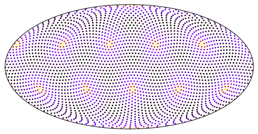
Matplotlib¶

Although pcolormesh won’t work, we can treat our data as scatter points or take advantage of Matplotlib’s tricontouring support.

fig, ax = plt.subplots(subplot_kw=dict(projection=ccrs.Mollweide()))

ax.set_global()

x = np.rad2deg(g.lonCell)
y = np.rad2deg(g.latCell)
data = g.areaCell

_ = ax.scatter(
    x,
    y,
    c=data,
    s=20,
    marker=".",
    linewidths=0,
    cmap="gnuplot_r",
    transform=ccrs.PlateCarree(),
)

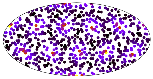
# The above becomes slow after 100k points or so,
# but you can still use it by slicing the data

fig, ax = plt.subplots(subplot_kw=dict(projection=ccrs.Mollweide()))

ax.set_global()

k = 4
_ = ax.scatter(
    x[::k],
    y[::k],
    c=data[::k],
    s=50,
    marker="o",
    linewidths=0,
    cmap="gnuplot_r",
    transform=ccrs.PlateCarree(),
)

from matplotlib.tri import Triangulation

# We can reuse this for different plots
# If we pass just x and y, a Delaunay triangulation is computed automatically
tri = Triangulation(x, y)
assert tri.is_delaunay
print(f"{len(tri.triangles)} triangles (real number: {g.sizes['nVertices']})")

fig, ax = plt.subplots(subplot_kw=dict(projection=ccrs.Mollweide()))

ax.set_global()

_ = ax.tricontourf(tri, data, levels=25, transform=ccrs.PlateCarree(), cmap="gnuplot_r")

5096 triangles (real number: 5120)

# For MPAS, we know that the dual mesh forms a Delaunay triangulation already
# and we can pass it, but the triangle defns have to be in CCW order
# Contouring technically takes values at grid points (mesh nodes),
# and the dual mesh nodes are the primal mesh centers
# The issue is that some of the triangles cross the antimeridian
# A more robust solution is to use
# https://mpas-dev.github.io/MPAS-Tools/1.0.0/generated/mpas_tools.viz.mesh_to_triangles.mesh_to_triangles.html
x = np.rad2deg(g.lonCell)
y = np.rad2deg(g.latCell)
inds = g.cellsOnVertex - 1
data = g.areaCell

tri = Triangulation(x, y, triangles=inds)
print(f"{len(tri.triangles)} triangles")

fig, ax = plt.subplots(subplot_kw=dict(projection=ccrs.Mollweide()), layout="constrained")

ax.set_global()

_ = ax.tricontour(tri, data, levels=25, transform=ccrs.Geodetic(), cmap="gnuplot_r")

5120 triangles

# The primal mesh edges connect the dual mesh centers
# but the primal mesh is not triangles (though each cell can be broken into tris)
# But we can use the auto triangulation
x = np.rad2deg(g.lonVertex)
y = np.rad2deg(g.latVertex)
data = g.areaTriangle

tri = Triangulation(x, y)
print(f"{len(tri.triangles)} triangles")

fig, ax = plt.subplots(subplot_kw=dict(projection=ccrs.Mollweide()), layout="constrained")

ax.set_global()

_ = ax.tricontour(tri, data, levels=15, transform=ccrs.PlateCarree(), cmap="gnuplot_r")

10217 triangles

uxarray¶

uxarray builds on xarray to provide a unified interface for working with unstructured-grid data, including MPAS.

uxarray considers the unit sphere internally.

uxg = ux.open_grid(grid_path)
uxds = ux.UxDataset.from_xarray(area.to_dataset(), uxgrid=uxg)

HoloViz¶

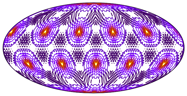
uxarray provides various routines for visualization with the help of HoloViews. By default, you get interactive plots that use the Bokeh backend. Rasterization, by datashader, can be explicitly turned on or off using the rasterize keyword (and configured using pixel_ratio).

uxg.plot(frame_width=450)

# More expensive, but we can fill the viewport
uxg.plot(periodic_elements="split", frame_width=450)

uxg.plot(projection=ccrs.Orthographic(), frame_width=450) * gf.coastline

%%time

# With high-resolution grids, rasterize=False can increase plot time significantly.
area = uxds.areaCell
proj = ccrs.Robinson()
cmap = "gnuplot_r"

layout = (
    area.plot.polygons(
        title="Vector polygons",
        projection=proj,
        periodic_elements="split",
        rasterize=False,
        line_width=0.5,
        line_color="0.5",
        cmap=cmap,
    )
    + area.plot.polygons(
        title="Default raster",
        projection=proj,
        periodic_elements="split",
        cmap=cmap,
    )
    + area.plot.polygons(
        title="Raster with pixel ratio 4",
        projection=proj,
        periodic_elements="split",
        pixel_ratio=4,  # > 1 to better resolve the cells
        cmap=cmap,
    )
)

layout.cols(1) * gf.coastline(line_color="limegreen")

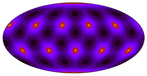
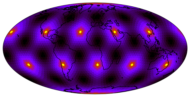
Raster¶

uxarray provides capabilities for generating raster representations of your data on the fly, for plotting with Cartopy/Matplotlib without needing to go through HoloViews. Here we also have pixel_ratio.

%%time

fig, ax = plt.subplots(subplot_kw=dict(projection=ccrs.Mollweide()), layout="constrained")

# Must set extent before calling `.to_raster()`
ax.set_global()

raster = uxds["areaCell"].to_raster(ax=ax)
ax.imshow(raster, cmap="gnuplot_r", origin="lower", extent=ax.get_xlim() + ax.get_ylim())
_ = ax.coastlines()

/home/runner/micromamba/envs/mpas-tutorial/lib/python3.12/site-packages/uxarray/grid/point_in_face.py:168: NumbaPerformanceWarning: np.dot() is faster on contiguous arrays, called on (Array(float64, 1, 'C', False, aligned=True), Array(float64, 1, 'A', False, aligned=True))
  hits = _get_faces_containing_point(

CPU times: user 10.7 s, sys: 406 ms, total: 11.1 s
Wall time: 8.4 s

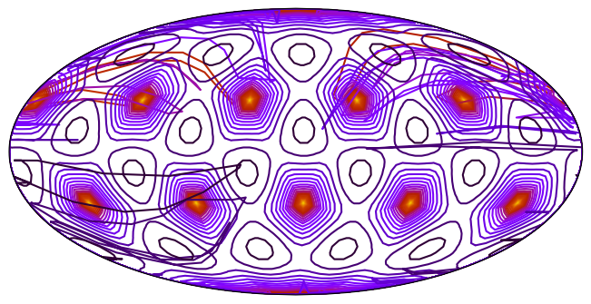
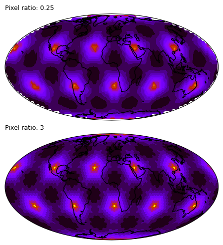
%%time

# The raster can also be contoured
# but with this very low-res data it's not really what we would want

fig, axs = plt.subplots(2, 1, subplot_kw=dict(projection=ccrs.Mollweide()), layout="constrained")

for ax, pixel_ratio in zip(axs.flat, [0.25, 3], strict=True):
    # Must set extent before calling `.to_raster()`
    ax.set_global()

    raster = uxds["areaCell"].to_raster(ax=ax, pixel_ratio=pixel_ratio)
    ax.contourf(
        raster,
        levels=30,
        cmap="gnuplot_r",
        origin="lower",
        extent=ax.get_xlim() + ax.get_ylim(),
    )
    ax.coastlines()
    ax.set_title(f"Pixel ratio: {pixel_ratio}", loc="left", size=9)

CPU times: user 15.8 s, sys: 100 ms, total: 15.9 s
Wall time: 4.72 s

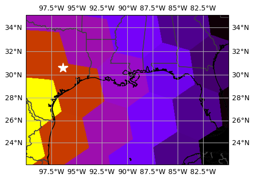
%%time

TAMU = -96.3364, 30.6187

fig, ax = plt.subplots(
    subplot_kw=dict(projection=ccrs.Mercator()), figsize=(5, 3.5), layout="constrained"
)

# Must set extent before calling `.to_raster()`
# The rasterization will be more efficient if we also select a spatial subset of the data,
# but it's not required
ax.set_extent((-100, -80, 22, 35))

raster = uxds["areaCell"].to_raster(ax=ax)
ax.imshow(raster, cmap="gnuplot_r", origin="lower", extent=ax.get_xlim() + ax.get_ylim())

ax.add_feature(cfeature.STATES, edgecolor="0.25", linewidth=1)
ax.coastlines()
ax.gridlines(draw_labels=True)

_ = ax.plot(*TAMU, marker="*", markersize=15, color="white", transform=ccrs.PlateCarree())

CPU times: user 2.86 s, sys: 5.92 ms, total: 2.87 s
Wall time: 846 ms

/home/runner/micromamba/envs/mpas-tutorial/lib/python3.12/site-packages/cartopy/io/__init__.py:242: DownloadWarning: Downloading: https://naturalearth.s3.amazonaws.com/10m_cultural/ne_10m_admin_1_states_provinces_lakes.zip
  warnings.warn(f'Downloading: {url}', DownloadWarning)

/home/runner/micromamba/envs/mpas-tutorial/lib/python3.12/site-packages/cartopy/io/__init__.py:242: DownloadWarning: Downloading: https://naturalearth.s3.amazonaws.com/10m_physical/ne_10m_coastline.zip
  warnings.warn(f'Downloading: {url}', DownloadWarning)

Matplotlib Collections¶

The meshes can also be represented exactly using Matplotlib Collections.

This is a good opportunity to use uxarray’s subsetting support, as Matplotlib Collections may be slow to plot if you provide too many cells.

lon_bounds = (-100, -80)
lat_bounds = (22, 35)
b = 5  # buffer for the selection so we can fill the plot area

fig, ax = plt.subplots(
    subplot_kw=dict(projection=ccrs.Mercator()), figsize=(5, 3.5), layout="constrained"
)

ax.set_extent(lon_bounds + lat_bounds)

# Here, especially if you have a large mesh, it is very beneficial to select
# the spatial subset first, to reduce the number of polygons computed/added
poly_collection = (
    uxds["areaCell"]
    .subset.bounding_box(
        lon_bounds=(lon_bounds[0] - b, lon_bounds[1] + b),
        lat_bounds=(lat_bounds[0] - b, lat_bounds[1] + b),
    )
    .to_polycollection()
)

poly_collection.set_cmap("gnuplot_r")
ax.add_collection(poly_collection)

ax.add_feature(cfeature.STATES, edgecolor="0.25", linewidth=1)
ax.coastlines()
ax.gridlines(draw_labels=True)

_ = ax.plot(*TAMU, marker="*", markersize=15, color="white", transform=ccrs.PlateCarree())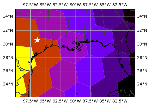

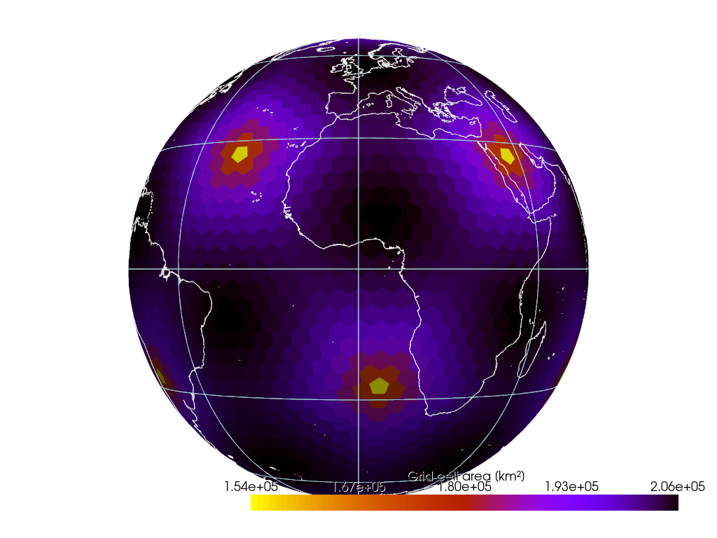
GeoVista¶

Built on PyVista/VTK, GeoVista provides GPU-accelerated interactive visualization of geospatial data and has builtin support for unstructured meshes.

It will still work if a GPU is not available/detected, but it may be much slower to first plot and to respond.

if not CI:
    conn = np.ma.masked_where(g.verticesOnCell == 0, g.verticesOnCell, copy=False) - 1

    mesh = gv.Transform.from_unstructured(
        np.rad2deg(g.lonVertex),
        np.rad2deg(g.latVertex),
        connectivity=conn,
        data=area,
    )

    pl = gv.GeoPlotter()

    sargs = {"title": r"Grid cell area [km²]", "shadow": True}
    pl.add_mesh(
        mesh,
        scalar_bar_args=sargs,
        cmap="gnuplot_r",
    )

    # pl.add_base_layer(texture=gv.natural_earth_hypsometric())
    pl.add_coastlines(color="white")
    pl.add_graticule(lon_step=None, lat_step=None, show_labels=False)

    pl.view_yz()
    pl.camera.zoom(1.5)

    pl.show()

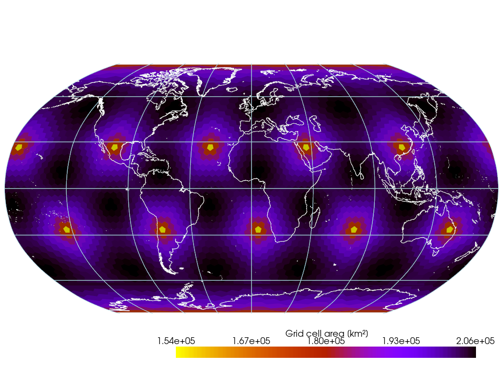
if not CI:
    pl = gv.GeoPlotter(crs="ESRI:54030")  # Robinson

    sargs = {"title": "Grid cell area [km²]", "shadow": True}
    pl.add_mesh(
        mesh,
        scalar_bar_args=sargs,
        cmap="gnuplot_r",
    )

    # pl.add_base_layer(texture=gv.natural_earth_hypsometric())
    pl.add_coastlines(color="white")
    pl.add_graticule(lon_step=None, lat_step=None, show_labels=False)

    pl.view_xy()
    pl.enable_image_style()  # better interactivity for 2-D plots
    pl.camera.zoom(1.5)

    pl.show()

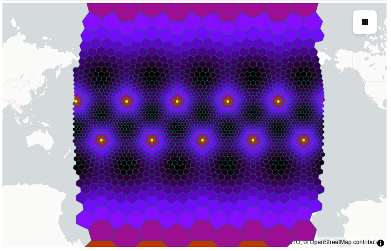
lonboard¶

lonboard provides GPU-accelerated interactive visualiation of geospatial vector data. We can pass it cell polygons. An easy way to get these is using uxarray.

from lonboard import Map, PolygonLayer
from matplotlib.colors import Normalize

gdf = (
    uxds["areaCell"]
    .to_geodataframe(engine="geopandas", periodic_elements="exclude")
    .set_crs("EPSG:4326")
)

arr = gdf.areaCell
cmap = plt.get_cmap("gnuplot_r")
norm = Normalize(vmin=arr.min(), vmax=arr.max())
colors = (cmap(norm(arr)) * 255).astype("uint8")

layer = PolygonLayer.from_geopandas(
    gdf,
    get_fill_color=colors,
    get_line_color=[0, 100, 100, 150],
    line_width_min_pixels=1,
)
m = Map(layer)
m

Footnotes¶

small files by default
↩
Or when this site is built, for that matter, which is why it is currently guarded.
↩